6 Hypothesis Testing
Hypothesis testing is a vital process in inferential statistics where the goal is to use sample data to draw conclusions about an entire population. A hypothesis test evaluates two mutually exclusive statements about a population to determine which statement is best supported by the sample data. These two statements are called the null hypothesis and the alternative hypothesis.
Why do we need a test? As mentioned, almost always in statistics, we are dealing with a sample instead of the full population. There are huge benefits when working with samples because it is usually impossible to collect data from an entire population. However, the trade off for working with a manageable sample is that we need to account for the sampling error. The sampling error is the gap between the sample statistic and the population parameter. Unfortunately, the value of the population parameter is not only unknown but usually unknowable. Hypothesis tests provide a rigorous statistical framework to draw conclusions about an entire population based on a representative sample.
As an example, given a sample mean of 350USD and a hypothetical population mean of 300USD, we can estimate how much is the probability that the population mean of 300USD is true (p-value), thus the sampling error, by using the T distribution (which is similar to the Normal Distribution, but with fattier tails). We will follow these four steps:
- First, we define the null (\(\bar i_n = \bar i_N\)) and alternative hypotheses (\(\bar i_n \neq \bar i_N\)). Much of the emphasis in classical statistics focuses on testing a single null hypothesis, such as H0: the average income between two groups is the same. Of course, we would probably like to discover that there is a difference between the average income in the two groups. But for reasons that will become clear, we construct a null hypothesis corresponding to no difference.
- Next, we construct a test statistic that summarizes the strength of evidence against the null hypothesis.
- We then compute a p-value that quantifies the probability of having obtained a comparable or more extreme value of the test statistic under the \(H_0\) (Lee 2019).
- Finally, based on a predefined significance level that we want to reach (alpha), we will decide whether to reject or not \(H_0\) that the population mean is 300.
Hypothesis tests are not 100% accurate because they use a random sample to draw conclusions about entire populations. When we perform a hypothesis test, there are two types of errors related to drawing an incorrect conclusion.
Type I error: rejects a null hypothesis that is true (a false positive).
Type II error: fails to reject a null hypothesis that is false (a false negative).
A significance level, also known as alpha, is an evidentiary standard that a researcher sets before the study. It defines how strongly the sample evidence must contradict the null hypothesis before we can reject the null hypothesis for the entire population. The strength of the evidence is defined by the probability of rejecting a null hypothesis that is true (Frost, n.d.). In other words, it is the probability that you say there is an effect when there is no effect. In practical terms, \(alpha=1-pvalue\). For instance, a p-value lower than 0.05 signifies 95% chances of detecting a difference between the two values. Higher significance levels require stronger sample evidence to be able to reject the null hypothesis. For example, to be statistically significant at the 0.01 requires more substantial evidences than the 0.05 significance level.
As mentioned, the significance level is set by the researcher. However there are some standard values that are conventionally applied in different scientific context, and we will follow these conventions.
| \(\alpha\) | \(p-value\) | symbol | scientific field |
|---|---|---|---|
| 80% | <0.2 | social science | |
| 90% | <0.1 | * | social science |
| 95% | <0.05 | ** | all |
| 99% | <0.01 | *** | all |
| 99.9% | <0.001 | physics |
Following we will see different type of tests, and their implementation using R. My suggestion, when working with really small numbers (such as the p-values), is to suppress the scientific notation in order to have a clearer sense of the coefficient scale. Use the following code.
6.1 Probability Distributions
All probability distributions can be classified as discrete probability distributions or as continuous probability distributions, depending on whether they define probabilities associated with discrete variables or continuous variables. With a discrete probability distribution, each possible value of the discrete random variable can be associated with a non-zero probability. Two of the most famous distributions associated with categorical data are the Binomial and the Poisson Distributions.
If a random variable is a continuous variable, its probability distribution is called a continuous probability distribution. This distribution differs from a discrete probability distribution because the probability that a continuous random variable will assume a particular value is zero, and the function that shows the density of the values of our data is called Probability Density Function, sometimes abbreviated pdf. Basically, this function represents the outline of the histogram. The probability that a random variable assumes a value between \(a\) and \(b\) is equal to the area under the density function bounded by \(a\) and \(b\) (Damodaran, n.d.).
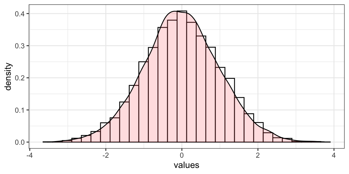
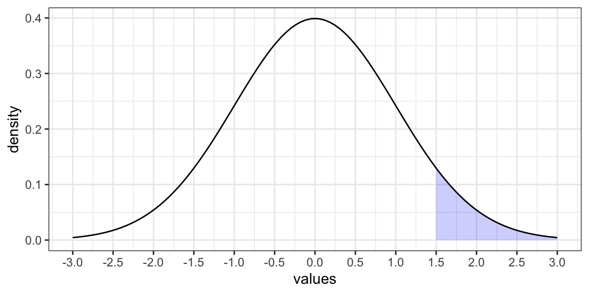
Figure 6.1: From left: A density distribution as outline of the hisogram; The probability that the random variable \(X\) is higher than or equal to 1.5.
In Figure 6.1, the shaded area in the graph represents the probability that the random variable \(X\) is higher than or equal to \(1.5\). This is a cumulative probability, also called p-value (please, remember this definition, as this will be key in order to understand all the remaining of this chapter). However, the probability that \(X\) is exactly equal to \(1.5\) would be zero.
The normal distribution, also known as the Gaussian distribution, is the most important probability distribution in statistics for independent, continuous, random variables. Most people recognize its familiar bell-shaped curve in statistical reports (Figure 6.1).
The normal distribution is a continuous probability distribution that is symmetrical around its mean, most of the observations cluster around the central peak, and the probabilities for values further away from the mean taper off equally in both directions.
Extreme values in both tails of the distribution are similarly unlikely. While the normal distribution is symmetrical, not all symmetrical distributions are normal. It is the most important probability distribution in statistics because it accurately describes the distribution of values for many natural phenomena (Frost, n.d.). As with any probability distribution, the parameters for the normal distribution define its shape and probabilities entirely. The normal distribution has two parameters, the mean and standard deviation.
Despite the different shapes, all forms of the normal distribution have the following characteristic properties.
They’re all symmetric bell curves. The Gaussian distribution cannot be skewed.
The mean, median, and mode are all equal.
One half of the population is less than the mean, and the other half is greater than the mean.
The Empirical Rule allows you to determine the proportion of values that fall within certain distances from the mean.
When we have normally distributed data, the standard deviation becomes particularly valuable. In fact, we can use it to determine the proportion of the values that fall within a specified number of standard deviations from the mean. For example, in a normal distribution, 68% of the observations fall within +/- 1 standard deviation from the mean (Figure 6.2). This property is part of the Empirical Rule, which describes the percentage of the data that fall within specific numbers of standard deviations from the mean for bell-shaped curves. For this reason, in statistics, when dealing with large-enough dataset, the normal distribution is assumed, even if it is not perfect.
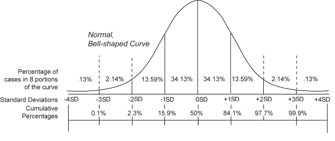
Figure 6.2: The Empirical Rule.
The standard normal distribution is a special case of the normal distribution where the mean is 0 and the standard deviation is 1. This distribution is also known as the Z-distribution. A value on the standard normal distribution is known as a standard score, or a Z-score. A standard score represents the number of standard deviations above or below the mean that a specific observation falls. A standard normal distribution is also the result of the z-score standardization process (see Scaling data)(Frost, n.d.). So, if we have to compare the means of the distributions of two elements (the weight of apple and pears), by standardizing we can do it (Figure 6.3).
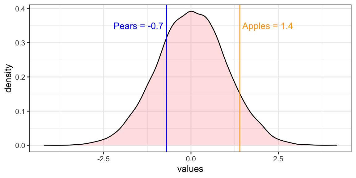
Figure 6.3: The comparison between Apples and Pears standardized.
6.2 Shapiro-Wilk Test
The Shapiro-Wilk Test is a way to tell if a random sample comes from a normal distribution. The test gives us a W value and a p-value. The null hypothesis is that our population is normally distributed. Thus, if we get a significant p-value (<0.1), we will have to reject \(H_0\), and we will consider the distribution as no normal. The test has limitations, most importantly it has a bias by sample size. The larger the sample, the more likely we will get a statistically significant result.
Why is it important to know if a random sample comes from a normal distribution? Because, if this hypothesis does not hold, we are not able to use the characteristics of the t-distribution in order to make some inference and, instead of using a T-Test, we will have to use a Wilcoxon Rank Sum test or Mann-Whitney test.
In order to perform a Shapiro-Wilk Test in R, we need to use the following code.
Code
6.3 One-Sample T-Test
One-Sample T-Test is used to compare the mean of one sample to a theoretical/hypothetical mean (as in our previous example). We can apply the test according to one of the three different type of hypotheses available, depending on our research question:
- The null hypothesis (\(H_0\)) is that the sample mean is equal to the known mean, and the alternative (\(H_a\)) is that they are not (argument “two.sided”).
- The null hypothesis (\(H_0\)) is that the sample mean is lower-equal to the known mean, and the alternative (\(H_a\)) is that it is bigger (argument “greater”).
- The null hypothesis (\(H_0\)) is that the sample mean is bigger-equal to the known mean, and the alternative (\(H_a\)) is that it is smaller (argument “less”).
In the code below, given an average consumption of 20.1 miles per
gallon, we want to test if the cars’ consumption is on average lower
than 22 miles per gallon (\(H_a\)). And this is in fact true, because we
retrieve a significant p-value (<0.05), thus we reject \(H_0\). By using
the package gginfernece (Bratsas, Foudouli, and Koupidis 2020), we can also plot this test.
Code
mean(mtcars$mpg)

# H0: cars consumption is on average 22 mpg or higher
# Ha: cars consumption is on average lower than 22 mpg
t.test(mtcars$mpg, mu = 22, alternative = "less")
#We reject H0. The average car consumption is significantly lower than 22 mpg.

# plot the t-test
library(gginference)
ggttest(t.test(mtcars$mpg, mu = 22, alternative = "less"))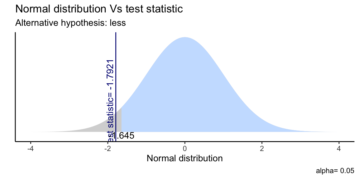
Figure 6.4: Single Sample T-Test as plotted by gginference package.
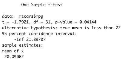
Figure 6.5: Single Sample T-Test output example.
The output of the test in R gives us many information. The most
important are: the data that we are using (mtcars$mpg), the t
statistics (if it is lower than 2, we have a significant p-value), the
p-value, the alternative hypothesis (\(H_a\)), the 95% confidence interval
(so the boundaries of 95% of the possible averages), and the sample
estimate of the mean.
6.4 Unpaired Two Sample T-Test
One of the most common tests in statistics is the Unpaired Two Sample T-Test, used to determine whether the means of two groups are equal to each other (Ziliak 2008). The assumption for the test is that both groups are sampled from normal distributions with equal variances. The null hypothesis (\(H_0\)) is that the two means are equal, and the alternative (\(H_a\)) is that they are not.
As an example, we can compare the average income between two group of
100 people. First, we explore some descriptive statistics about the two
groups in order to have an idea. And we see that the difference between
the two groups is only 0.69. Note, that we set the seed because we
generate our data randomly from an Normal distribution using the
function rnorm().
Code
Before proceeding with the test, we should verify the assumption of normality by doing a Shapiro-Wilk Test as explained before. However, as the data are normally distributed by construction, we will skip this step.
We will then state our hypotheses, and run the Unpaired Two Sample
T-Test. The R function is the same as for the One-Sample T-Test, but
specifying different arguments. We can again plot our test using the
package gginfernece (Bratsas, Foudouli, and Koupidis 2020).
Code
# H0: the two groups have the same income on average
# Ha: the two groups have the different income on average
t.test(income_a, income_b) # reject H0
# We accept Ha. There is a SIGNIFICANT mean income difference (0.67)
# between the two groups.

library(gginference)
ggttest(t.test(income_a, income_b))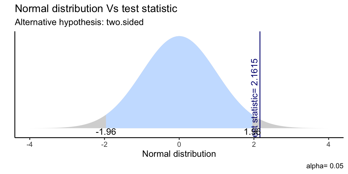
Figure 6.6: Single Sample T-Test as plotted by gginference package.
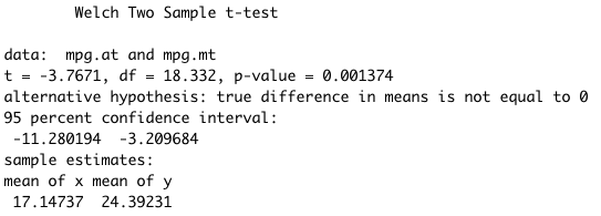
Figure 6.7: Two sample T-test output example.
As for the One-Sample T-Test, R gives us a set of information about the test. The most important are: the data that we are using, the t statistics (if it is lower than 2, we have a significant p-value), the p-value, the alternative hypothesis (\(H_a\)), the 95% confidence interval (so the boundaries of 95% of the possible difference between the averages of the two groups), and the sample estimates of the mean. Note that we will have to compute the difference between the two averages “by hand”, in case we needed.
If we want to extract the coefficients, the p-value or any other information given by the t-test in order to build a table, we must assign the test to an object first, and then extract the data. In the code below we run the Unpaired Two Sample T-Test for manual and automatic on the average consumption and weight of the cars. We then create a table with the average difference and the p-value of both tests. Note that the t-test formula is written in a different way than in the code chunk above, however the meaning of the two expressions is the same.
Code
6.5 Mann Whitney U Test
In the case the variable we want to compare are not normally distributed (aka: the Shapiro test gives us a significant p-value), we can run a Mann Whitney U Test, also known as Wilcoxon Rank Sum test (Winter 2013). It is used to test whether two samples are likely to derive from the same population (i.e., that the two populations have the same shape). Some scholars interpret this test as comparing the medians between the two populations. Recall that the Unpaired Two Sample T-Test compares the means between independent groups. In contrast, the research hypotheses for this test are stated as follows:
\(H_0\): The two populations are equal versus
\(H_a\): The two populations are not equal.
The procedure for the test involves pooling the observations from the two samples into one combined sample, keeping track of which sample each observation comes from, and then ranking lowest to highest.
In order to run it, the only thing we need to change is the name of the formula of the test, as written in the code below.
6.6 Paired Sample T-Test
The Paired Sample T-Test is a statistical procedure used to determine whether the mean difference between two sets of observations is zero. Common applications of the Paired Sample T-Test include case-control studies or repeated-measures designs (time series). In fact, each subject or entity must be measured twice, resulting in pairs of observations. As an example, suppose we are interested in evaluating the effectiveness of a company training program. We would measure the performance of a sample of employees before and after completing the program, and analyze the differences using a Paired Sample T-Test to see its impact.
The code below generates a dataset with some before and after values. We then compute the difference between the two measures and run a Shapiro-Wilk Test on them in order to verify the normality of the data distribution. Finally, we can run the proper Paired Sample T-Test on our data (or a Paired Mann Whitney U Test, if data are not normally distributed).
Code
df <- data.frame("before" = c(200.1, 190.9, 192.7, 213, 241.4, 196.9,
                              172.2, 185.5, 205.2, 193.7),
                 "after" = c(392.9, 393.2, 345.1, 393, 434, 427.9, 422,
                             383.9, 392.3, 352.2))

# compute the difference
df$difference <- df$before - df$after
# H0: the variables are normally distributed
shapiro.test(df$difference) # accept H0
hist(df$difference)

t.test(df$before, df$after, paired = TRUE)